Context

Note

This tutorial is based on our article Asymptotic ultimate regime of homogeneous Rayleigh–Bénard convection on logarithmic lattices. For more information, refer to the paper.

Rayleigh-Bénard

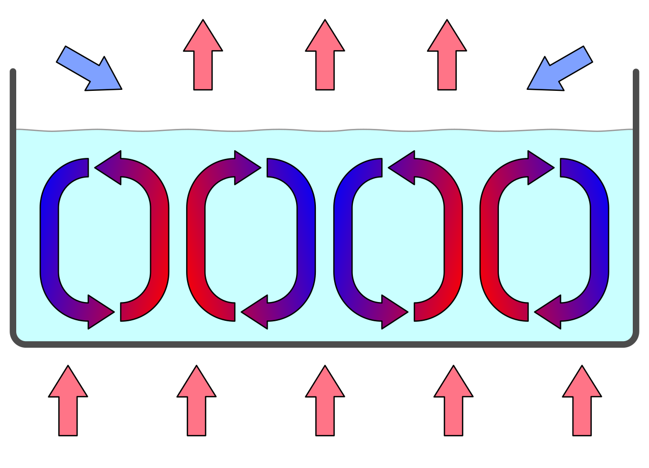
Rayleigh-Bénard equations describe the evolution of a volume of fluid heated from below in a container, and read in their basic form:

\(\nabla \cdot \mathbf{u} = 0\)

\(\frac{\partial \mathbf{u}}{\partial t} + (\mathbf{u} \cdot \nabla) \mathbf{u} = -\frac{1}{\rho} \nabla p + \nu \nabla^2 \mathbf{u} + \mathbf{g} \alpha (T - T_0)\)

\(\frac{\partial T}{\partial t} + \mathbf{u} \cdot \nabla T = \kappa \nabla^2 T\)

where \(u\) is the velocity, \(p\) the pressure, \(\rho\) the density, \(\nu\) the kinematic viscosity, \(\mathbf{g}\) the acceleration due to gravity, \(\alpha\) the thermal expansion coefficient, \(T\) the temperature, \(T_0\) a reference temperature, \(\kappa\) the thermal diffusivity.

(Homogeneous) Rayleigh-Bénard on Log-lattices

Standard Rayleigh-Bénard equations can’t be translated as-is on Log-lattices, because:

1. the term \(\mathbf{g} \beta (T - T_0)\) doesn’t nicely convert to a finite Fourier expansion

2. the boundary conditions (heated from below, in a container) can’t be represented in finite Fourier space either, which only accepts periodic boundary conditions.

Therefore, we instead simulate Homogeneous Rayleigh-Bénard (HRB), which corresponds to the following set of equations:

\(\nabla \cdot \mathbf{u} = 0\)

\(\frac{\partial \mathbf{u}}{\partial t} + (\mathbf{u} \cdot \nabla) \mathbf{u} = -\frac{1}{\rho} \nabla p + \nu \nabla^2 \mathbf{u} + \mathbf{g} \alpha \theta \mathbf{z}\)

\(\frac{\partial T}{\partial t} + \mathbf{u} \cdot \nabla T = \kappa \nabla^2 T + u_z\frac{\Delta T}{H}\)

where \(\theta\) is the temperature fluctuation relative to an affine profile, \(\Delta T\) the mean imposed temperature gradient, \(H\) the height of the container, \(\mathbf{z}\) the vertical unit vector.

Using the Rayleigh number \(Ra=\alpha gH^3\Delta T/(\nu\kappa)\) and the Prandl number \(Pr=\nu/\kappa\), those can be rewritten in adimentionalized form

\(\partial_t u_i = \mathbb{P}\left[-u_j\partial_ju_i+\frac{Pr}{Ra}\nabla^2u_i-fu_i\delta_{k\approx k_{min}}\right]_i\)

\(\partial_t\theta_i = -u_i\partial_i\theta + u_z + \frac{\nabla^2\theta}{\sqrt{RaPr}}-f\delta_{k\approx k_{min}}\)

where \(\mathbb{P}(A)=A-(k_i/k^2)k_jA_j\) is a projector that accounts for the pressure term under divergence-free conditions, and \(f\delta_{k\approx k_{min}}\) is an additional friction term that suppresses exponential instabilities (read the article for more detail and justification).